OpenPrescribing Seasonality Detection Pipeline

Author

Nasir Abdulrasheed

Introduction

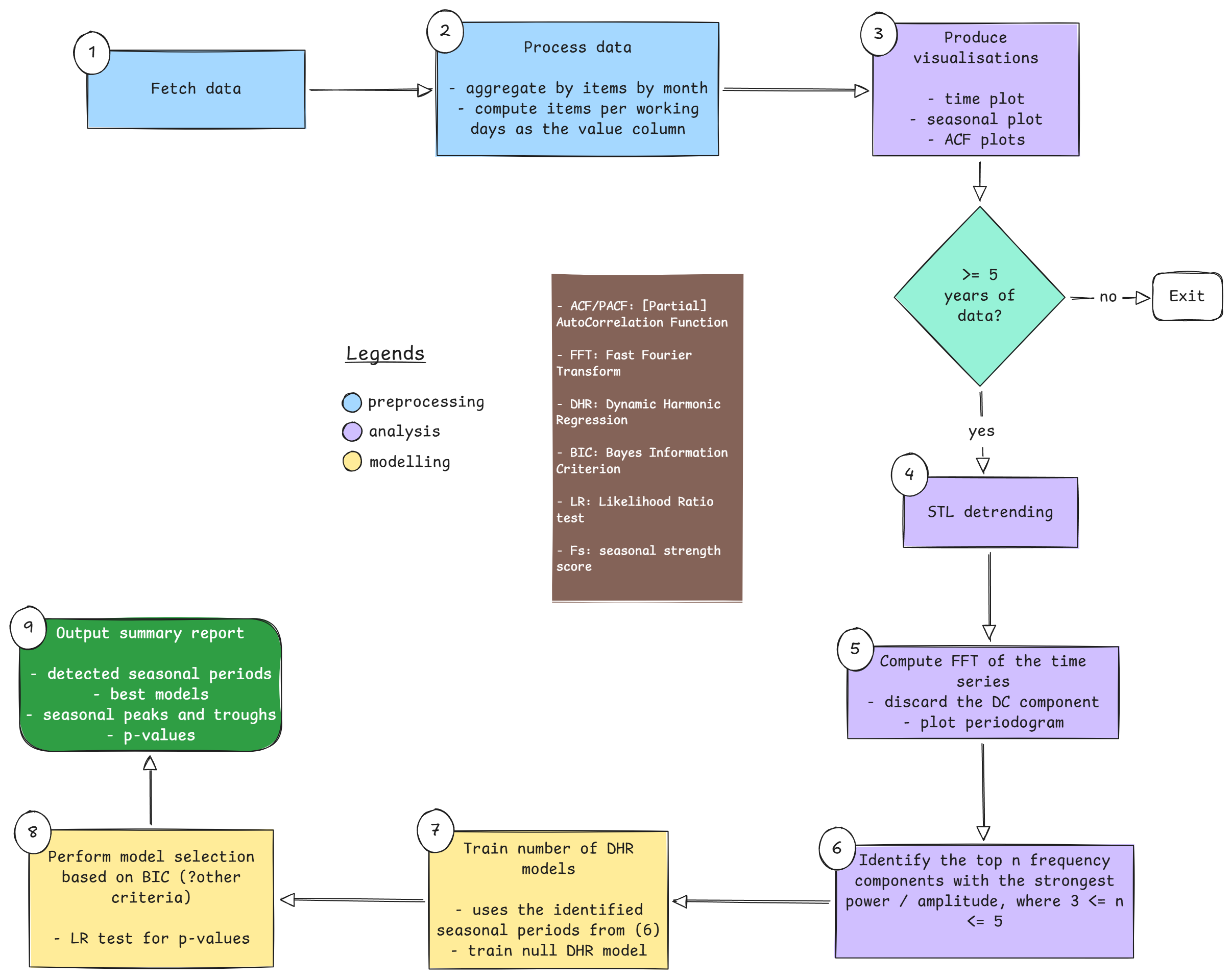
The aim of this project is to create a robust pipeline in R that automates the detection of seasonal patterns in English prescribing using data from OpenPrescribing. The ten steps of the pipeline are depicted in Figure 1.

Figure 1: Seasonality detector pipeline
Code
library(tidyverse)
library(arrow)
library(gt)
library(webshot2)
library(fpp3)
library(bizdays)
library(timeDate)
library(patchwork)
library(here)
library(glue)
library(purrr)
library(urca)
library(ggrepel)

MAX_PRODUCTS <- Inf

SERTRALINE_HCL <- "0403030Q0"
ESCITALOPRAM <- "0403030X0"
LORATADINE <- "0304010D0"
FEXOFENADINE_HCL <- "0304010E0"

PLOTS_DIR <- "outputs/nasir/figures"
TBL_DIR <- "outputs/nasir/tables"

DETREND_TYPE <- "stl"

DATE_START <- "2016-05-01"
DATE_END <- "2026-04-01"

Step 1: Load data

Loading data from disk. Table 1 shows the expected shape of the data expected to be fed into the pipeline.

Code
dev_drugs_file <- glue("df_dev_drugs_{DATE_START}_{DATE_END}.parquet")
DF_PRESC <- read_parquet(here("data-raw", "nasir", dev_drugs_file))

N_MONTHS <- unique(DF_PRESC$month) |> length()
N_YEAR_MONTHS <- 12 * (N_MONTHS %/% 12)

head(DF_PRESC, 5) |> gt()
Table 1: Monthly prescribing data for select drugs (May 2016 to April 2026)
sha regional_team stp pct practice bnf_code bnf_name items quantity month year_month chapter section para subpara chemical product chemical_code
QHM Y63 QHM 16C A81002 0403030X0AAAAAA Escitalopram 10mg tablets 24 742 2023-09-01 2026-06 Central Nervous System Antidepressant drugs Selective serotonin re-uptake inhibitors Selective serotonin re-uptake inhibitors Escitalopram Escitalopram 0403030X0
QHM Y63 QHM 16C A81012 0403030Q0AAABAB Sertraline 100mg tablets 219 6685 2023-09-01 2026-06 Central Nervous System Antidepressant drugs Selective serotonin re-uptake inhibitors Selective serotonin re-uptake inhibitors Sertraline hydrochloride Sertraline hydrochloride 0403030Q0
QHM Y63 QHM 16C A81016 0304010E0AAAAAA Fexofenadine 120mg tablets 64 1839 2023-09-01 2026-06 Respiratory System Antihistamines, hyposensitisation and allergic emergencies Antihistamines Antihistamines Fexofenadine hydrochloride Fexofenadine hydrochloride 0304010E0
QHM Y63 QHM 16C A81016 0304010E0AAABAB Fexofenadine 180mg tablets 83 3183 2023-09-01 2026-06 Respiratory System Antihistamines, hyposensitisation and allergic emergencies Antihistamines Antihistamines Fexofenadine hydrochloride Fexofenadine hydrochloride 0304010E0
QHM Y63 QHM 16C A81021 0403030Q0AAABAB Sertraline 100mg tablets 753 20103 2023-09-01 2026-06 Central Nervous System Antidepressant drugs Selective serotonin re-uptake inhibitors Selective serotonin re-uptake inhibitors Sertraline hydrochloride Sertraline hydrochloride 0403030Q0

The data used spans exactly 120 months (10 years).

Step 2: Preprocessing

To normalise total monthly items, the number of dispensing days in each month in the data was computed:

\[ N_{dispensing\_days} = Total\_Days - Sundays - Bank\_Holidays \tag{1}\]

Code
# bank holidays in the data period
uk_holidays <- as.Date(holidayLONDON(year(DATE_START):year(DATE_END)))

dispensing_days <- create.calendar(
  name = "UK",
  weekdays = c("sunday"),
  holidays = uk_holidays
)

month_work_days <- function(date) {
  month_start <- as.Date(date)
  month_end <- seq(month_start, by = "month", length.out = 2)[2] - 1
  length(bizseq(month_start, month_end, dispensing_days))
}

The data is then aggregated by month, chemical_code, and chemical columns to create a monthly items_per_wd column that holds the total items of that chemical dispensed in a given month across English primary care, normalised by the number of dispensing days. Table 2 shows a sample of the resulting data following aggregation.

Code
aggregate_ts <- function(df) {
  df |>
    summarise(
      total_items = sum(items),
      .by = c(month, chemical_code, chemical)
    ) |>
    mutate(month = yearmonth(month)) |>
    as_tsibble(index = month, key = c(chemical, chemical_code)) |>
    mutate(items_per_wd = total_items / map_dbl(month, month_work_days))
}
Code
DF_PRESC_AGG <- aggregate_ts(DF_PRESC)
df_sertraline <- filter(DF_PRESC_AGG, chemical_code == SERTRALINE_HCL)
df_escitalopram <- filter(DF_PRESC_AGG, chemical_code == ESCITALOPRAM)
df_loratadine <- filter(DF_PRESC_AGG, chemical_code == LORATADINE)
df_fexofenadine <- filter(DF_PRESC_AGG, chemical_code == FEXOFENADINE_HCL)

head(DF_PRESC_AGG, 5) |> gt()
Table 2: Sample of aggregated time series data
month chemical_code chemical total_items items_per_wd
2016 May 0403030X0 Escitalopram 78457 3269.042
2016 Jun 0403030X0 Escitalopram 81405 3130.962
2016 Jul 0403030X0 Escitalopram 80111 3081.192
2016 Aug 0403030X0 Escitalopram 80653 3102.038
2016 Sep 0403030X0 Escitalopram 82098 3157.615

Step 3: Visualisation

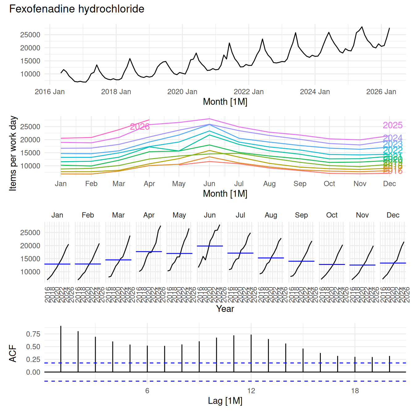
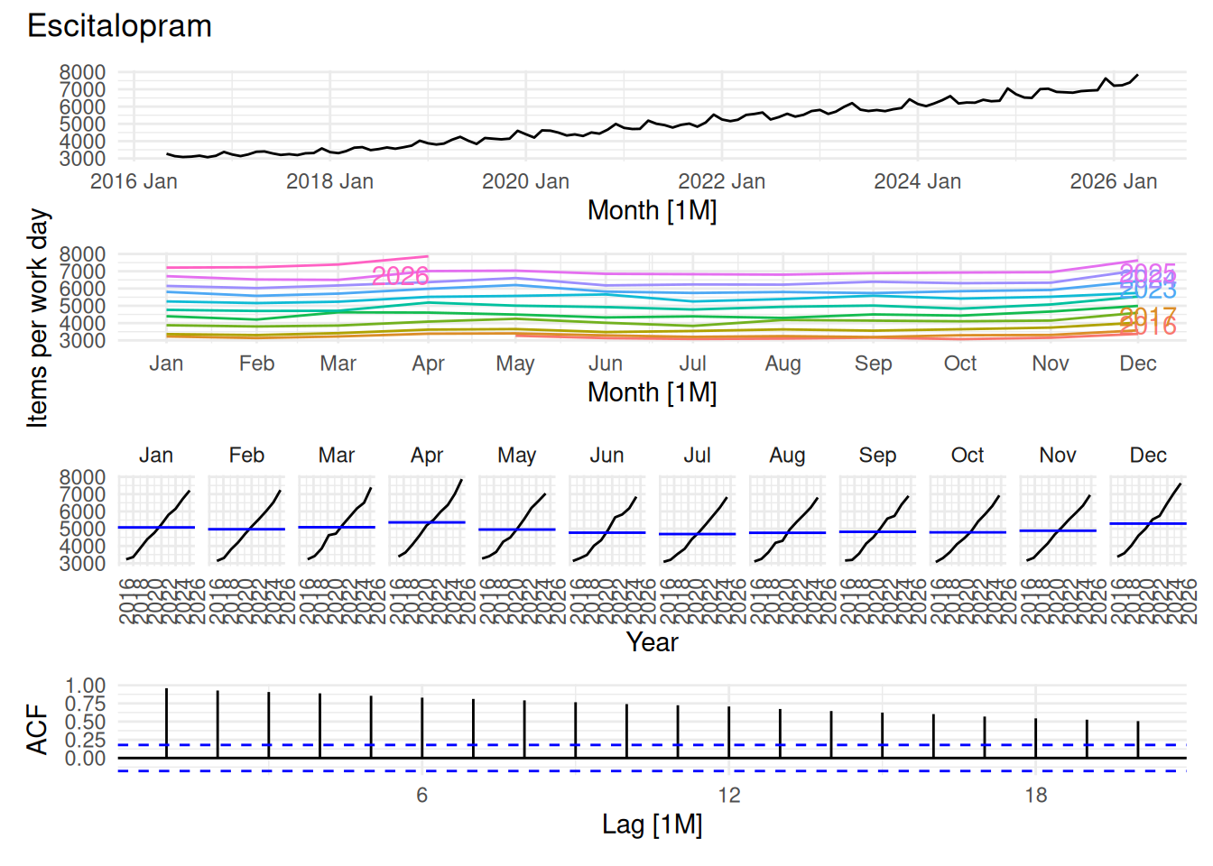
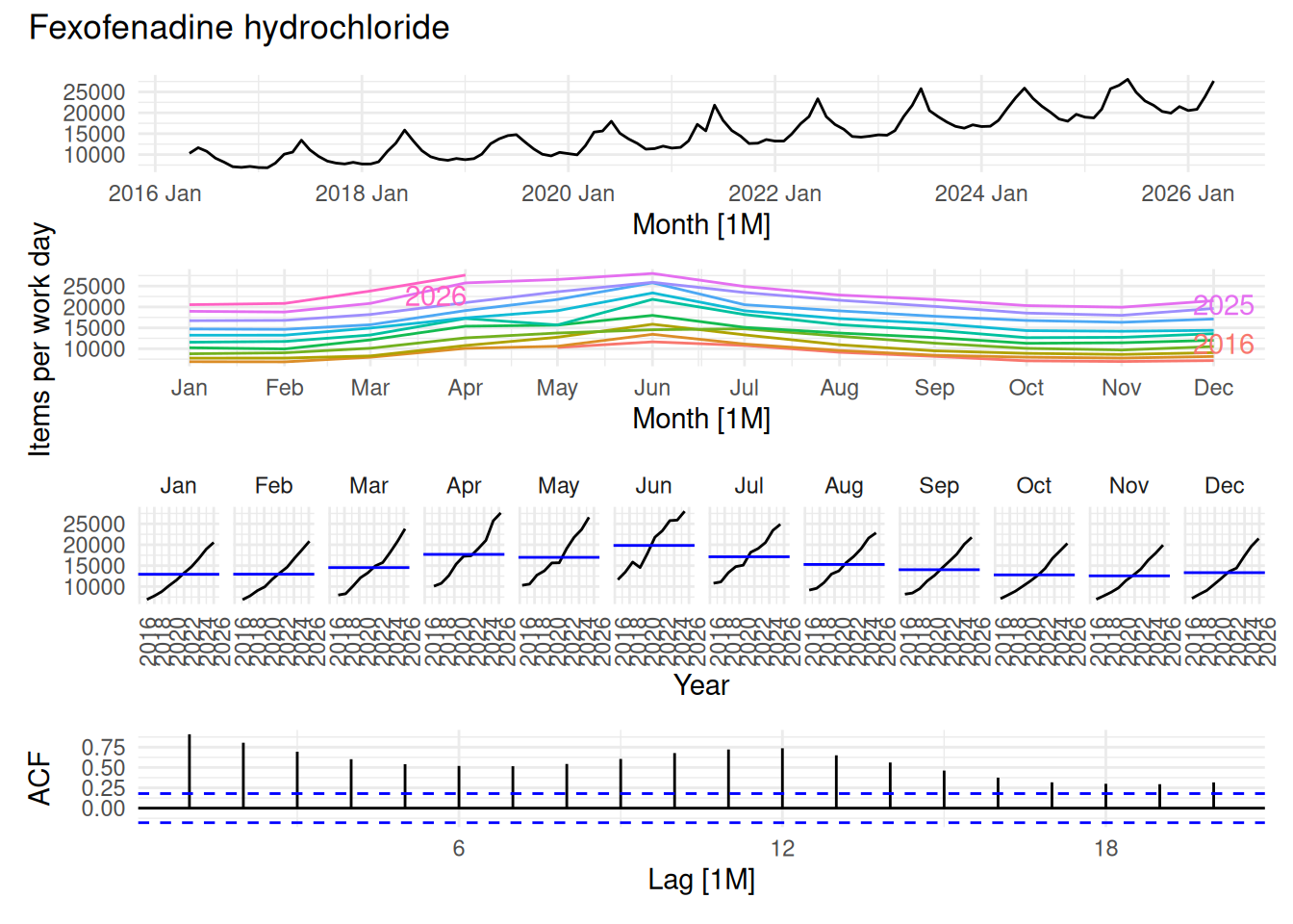
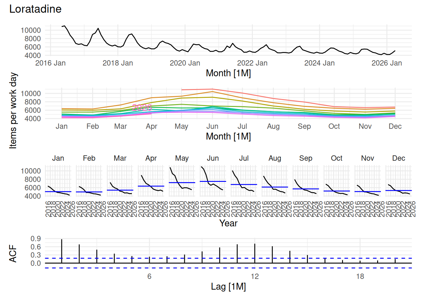
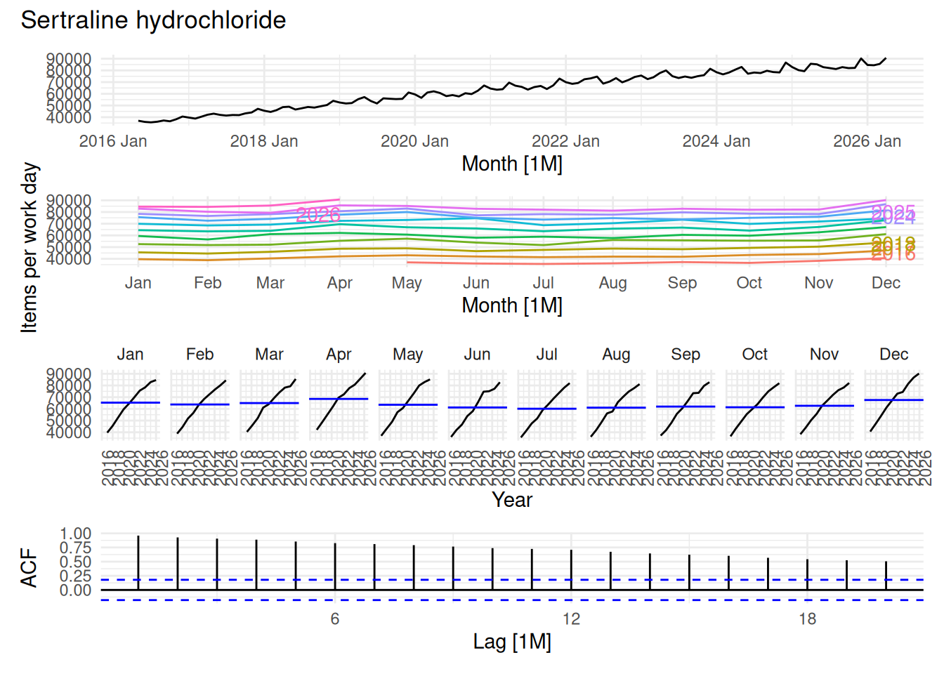
For all chemicals present in the data, we plotted time, seasonal, seasonal subseries, and ACF plots.

Code
visualise_ts <- function(ts) {
  if (!inherits(ts, "tbl_ts")) {
    stop("Argument `ts` must be a time series object")
  }

  chems <- unique(ts$chemical)
  plots <- list()
  for (i in seq_along(chems)) {
    chem <- chems[i]
    chem_ts <- filter(ts, chemical == chem)
    time_plot <- chem_ts |>
      autoplot(items_per_wd) +
      theme(legend.position = "none") +
      theme_minimal() +
      labs(y = "Items per work day", x = "Month [1M]")

    seasonal_plot <- chem_ts |>
      gg_season(
        items_per_wd,
        labels = "right",
        labels_repel = TRUE
      ) +
      theme_minimal() +
      labs(y = "Items per work day", x = "Month [1M]")

    subseries_plot <- chem_ts |>
      gg_subseries(items_per_wd) +
      theme_minimal() +
      theme(
        axis.text.x = element_text(angle = 90, hjust = 1),
        strip.text.y = element_blank(),
        strip.background = element_blank()
      ) +
      labs(y = "Items per work day", x = "Year")

    acf_plot <- chem_ts |>
      ACF(items_per_wd) |>
      autoplot() +
      theme_minimal() +
      labs(y = "ACF", x = "Lag [1M]")

    p <- (time_plot / seasonal_plot / subseries_plot) +
      plot_layout(axis_titles = "collect_y")
    p <- (p / acf_plot) +
      plot_annotation(title = chem)

    save_file <- glue("{chem}_plots_{DATE_START}_{DATE_END}.png")
    ggsave(
      here(PLOTS_DIR, save_file),
      width = 7,
      height = 7,
      units = "in"
    )

    print(p)
  }
}

Figure 2 shows the output of the visualising function for one chemical (Sertraline Hydrochloride, BNF code 0403030Q0).

Code
visualise_ts(df_fexofenadine)
Figure 2: Example output plots

Step 4: Detrending

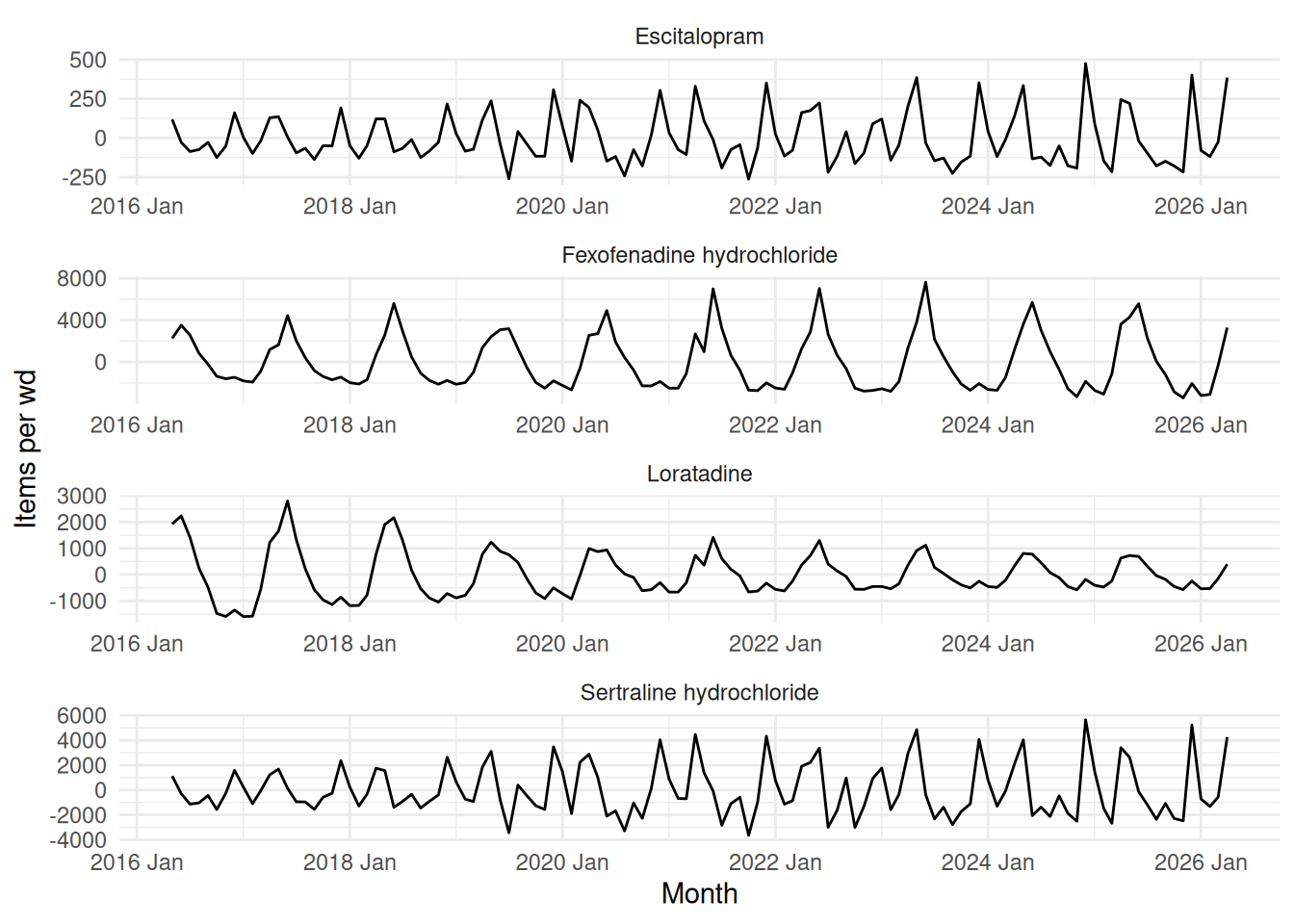
In this step, the detrended time series is obtained from either an STL decompoisition, LOESS, or linear model of the original time series. All three methods were tested and the results compared. The detrended series is then plotted as shown in Figure 7. Seasonal strength scores, trough and peak months are also computed using the feats::feat_stl() function.

Code
detrend_stl <- function(ts, s.window = 13) {
  DETREND_TYPE <<- "stl"

  ts |>
    model(
      STL(items_per_wd ~ trend() + season(window = s.window))
    ) |>
    components() |>
    mutate(detrended = season_year + remainder) |>
    select(chemical, chemical_code, month, detrended, season_year)
}

detrend_linear <- function(ts) {
  # simple linear time trend
  DETREND_TYPE <<- "linear"

  ts |>
    model(linear_trend = TSLM(items_per_wd ~ trend())) |>
    augment() |>
    select(chemical, chemical_code, month, detrended = .resid)
}

detrend_loess <- function(ts, span = 0.75) {
  # plain loess detrending
  DETREND_TYPE <<- "loess"

  ts |>
    as_tibble() |>
    group_by(chemical, chemical_code) |>
    mutate(
      t = row_number(),
      # Fit the Loess curve and extract the fitted trend line
      trend_curve = loess(items_per_wd ~ t, span = span)$fitted,
      detrended = items_per_wd - trend_curve
    ) |>
    ungroup() |>
    select(-t, -trend_curve) |>
    as_tsibble(index = month, key = c(chemical, chemical_code))
}

plot_decomp <- function(ts, s.window = 13) {
  chems <- unique(ts$chemical)
  decomp_plots <- list()

  for (i in seq_along(chems)) {
    chem <- chems[[i]]
    decomp <- ts |>
      filter(chemical_code == chem) |>
      model(
        STL(items_per_wd ~ trend() + season(window = s.window))
      ) |>
      components()

    p1 <- decomp |>
      autoplot(items_per_wd) +
      theme_minimal() +
      labs(title = chem, y = "Items per work day")

    p2 <- decomp |>
      ACF(remainder) |>
      autoplot() +
      theme_minimal() +
      labs(y = "ACF", x = "Lag [1M]")

    p <- (p1 / p2) + plot_layout(heights = c(0.75, 0.25))
    ggsave(
      here(PLOTS_DIR, glue("decomp_plots_{chem}.png")),
      width = 7,
      height = 7,
      units = "in"
    )

    decomp_plots[[i]] <- p
  }

  decomp_plots
}

detrended_plots <- function(ts_detrend) {
  rows <- length(unique(ts_detrend$chemical))
  p <- ggplot(ts_detrend) +
    geom_line(aes(x = month, y = detrended)) +
    facet_wrap(~chemical, scales = "free", nrow = rows) +
    theme_minimal() +
    theme(legend.position = "none") +
    labs(
      x = "Month",
      y = "Items per wd"
    )

  ggsave(here(PLOTS_DIR, glue("detrended_plots_{DETREND_TYPE}.png")))

  p
}

seasonal_comp_plots <- function(ts_detrend) {
  if (DETREND_TYPE != "stl") {
    return(invisible())
  }

  rows <- length(unique(ts_detrend$chemical))
  p <- ggplot(ts_detrend) +
    geom_line(aes(x = month, y = season_year)) +
    facet_wrap(~chemical, scales = "free", nrow = rows) +
    theme_minimal() +
    theme(legend.position = "none") +
    labs(
      x = "Month",
      y = "Items per wd"
    )

  ggsave(
    here(PLOTS_DIR, glue("seasonal_comp_plots_{DETREND_TYPE}.png"))
  )

  p
}

strength_stl <- function(ts_agg) {
  FIRST_MONTH <- ts_agg |>
    slice_head(n = 1) |>
    pull(month) |>
    month()

  results <- ts_agg |>
    features(items_per_wd, feat_stl) |>
    select(-spikiness, -linearity, -curvature, -starts_with("stl_")) |>
    mutate(
      seasonal_peak = month.abb[
        ((FIRST_MONTH - 2 + seasonal_peak_year) %% 12) + 1
      ],
      seasonal_trough = month.abb[
        ((FIRST_MONTH - 2 + seasonal_trough_year) %% 12) + 1
      ]
    ) |>
    select(-seasonal_peak_year, -seasonal_trough_year)

  write_parquet(
    results,
    here(TBL_DIR, "strength_scores.parquet")
  )

  results
}

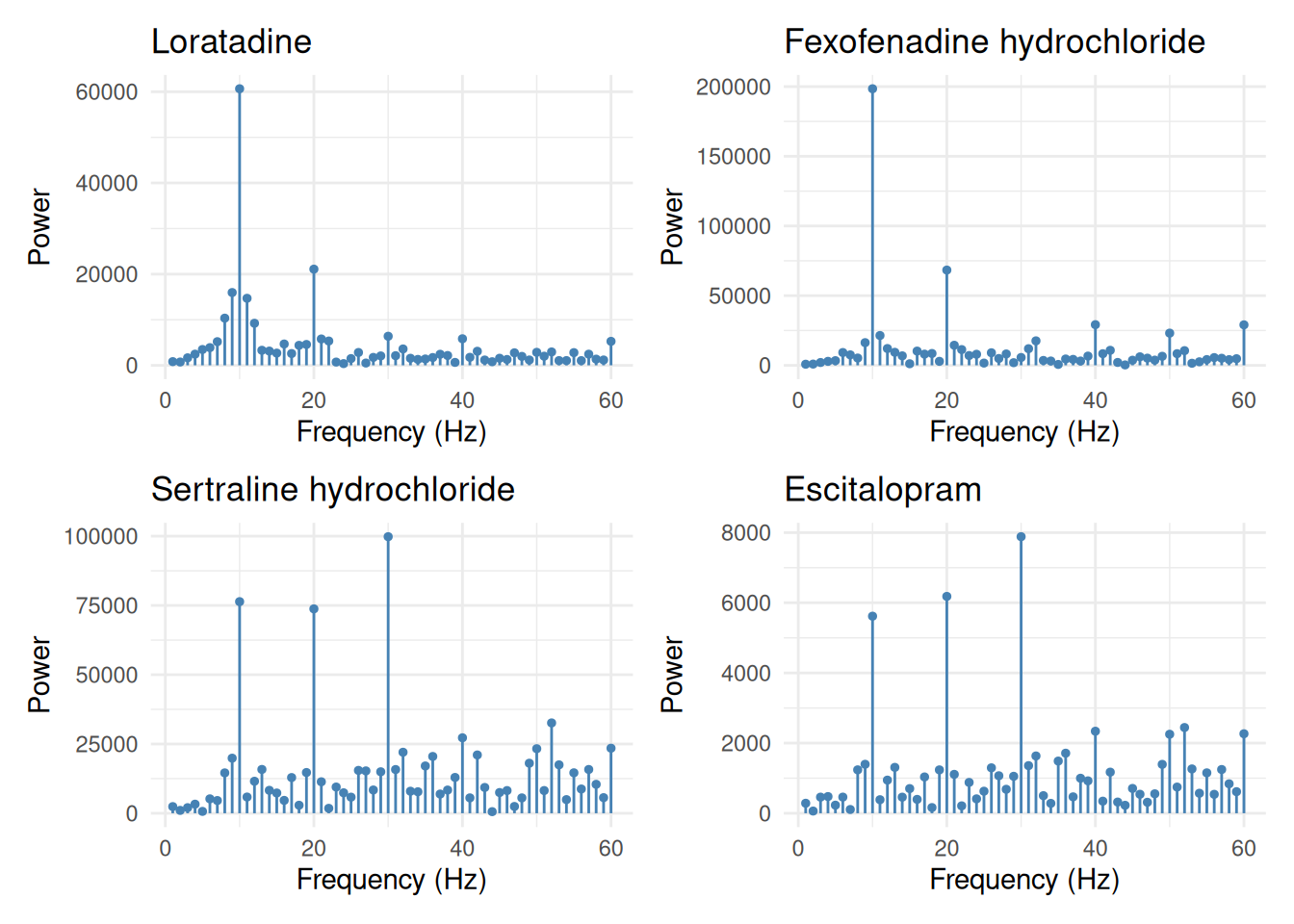
Step 5 & 6: FFT filtering and candidate periods selection

A fast fourier transform (FFT) of the detrended time series is taken to see the component signals (seasonalities) and their respective amplitudes/strength. For computing the FFT of the series, we use the last \(N\) months of the series that makes up full years. \(N\) is given by:

\[ N = 12 \left\lfloor \frac{total\ months}{12} \right\rfloor \tag{2}\] After computing the FFT, we only keep the coefficients for periods bins between 2 and 24 months. This is because the Nyquist for monthly data is 0.5 Hz (2 months) and we are mostly interested in annual and subannual seasonalities.

Code
compute_fft <- function(ts) {
  if (!is.vector(ts)) {
    stop("Argument `ts` must be a vector")
  }

  len_ts <- length(ts)

  ts <- ts[(len_ts - N_YEAR_MONTHS):len_ts]
  len_ts <- N_YEAR_MONTHS / 2

  amps <- fft(ts) |> abs()

  amps[2:(len_ts + 1)]
}

filter_fft <- function(fft_amps, top_k = 1) {
  if (!is.vector(fft_amps)) {
    stop("Argument `fft_amps` must be a vector")
  }

  if (top_k > length(fft_amps)) {
    stop("`top_k` cannot exceed the length of `fft_amps` amplitudes vector")
  }

  sort_idx <- order(fft_amps, decreasing = TRUE)
  min_freq <- N_YEAR_MONTHS %/% 24
  max_freq <- N_YEAR_MONTHS %/% 2
  sort_idx <- sort_idx[(sort_idx >= min_freq) & (sort_idx <= max_freq)]
  candidates <- sort_idx[1:top_k]
  amps <- fft_amps[candidates]

  list(freqs = candidates, amps = amps)
}

plot_fft <- function(fft_amps, chemical) {
  if (!is.vector(fft_amps)) {
    stop("Argument `fft_amps` must be a vector")
  }

  len_ts <- length(fft_amps)

  freqs <- 1:len_ts

  spectral_plot <- ggplot(mapping = aes(x = freqs, y = fft_amps)) +
    geom_segment(
      aes(xend = freqs, y = 0, yend = fft_amps),
      colour = "steelblue"
    ) +
    geom_point(colour = "steelblue", size = 1) +
    theme_minimal() +
    labs(
      x = "Frequency (Hz)",
      y = "Power",
      title = chemical
    )

  save_file <- glue("{chemical}_fft_{DETREND_TYPE}_{DATE_START}_{DATE_END}.png")
  ggsave(
    here(PLOTS_DIR, save_file),
    width = 7,
    height = 7,
    units = "in"
  )

  spectral_plot
}

Figure 9 shows the periodograms for the chemicals in the current data. It shows the frequecies/wave number of the seasonal signals present in the time series, along with their respective amplitdes/power. The seasonal period, \(p\), which is the number of month after which the seasonal signal repeats is given by:

\[ p = N / f \tag{3}\] where \(N\) is the number of months from Equation 2 and \(f\) is the frequenc/wave number from the x axis of the periodograms. So for frequency 10, seasonal period is \(120 / 10 = 12\ months\), for frequency 20, \(p\) is \(120 / 20 = 6\ months\), etc.

Code
score <- function(ts_dable, top_k = 1) {
  chems <- unique(ts_dable$chemical)
  scores <- tibble()
  plots <- list()

  for (i in seq_along(chems)) {
    chem <- chems[i]
    chem_dable <- ts_dable |>
      filter(chemical == chem)

    fft_amps <- chem_dable |>
      pull(detrended) |>
      compute_fft()

    plots[[i]] <- plot_fft(fft_amps, chem)

    amps_freqs <- filter_fft(fft_amps, top_k)
    tmp_df <- tibble(chemical = chem)

    for (j in seq_along(amps_freqs$freqs)) {
      col_period <- paste0("period_", j)
      col_freq <- paste0("freq_", j)
      col_score <- paste0("score_", j)

      tmp_df <- bind_cols(
        tmp_df,
        tibble(
          "{col_period}" := round(N_YEAR_MONTHS / amps_freqs$freqs[j], 2),
          "{col_freq}" := round(amps_freqs$freqs[j], 2),
          "{col_score}" := amps_freqs$amps[j]
        )
      )
    }

    scores <- bind_rows(scores, tmp_df)
  }

  list(plots = plots, scores = scores)
}

Step 7 & 8: DHR Modelling and Selection

In this step, we fit Dynamic Harmonic Regression(DHR) models to the aggregated time series data. Each model uses the each candidate period (\(p\)) as its fundamental frequency/period and set \(K\) (the number of harmonics to include) to be a maximum of \(p // 2\) (its Nyquist). Therefore, the maximum number of models fitted is given by:

\[ N \leq \sum_{i=1}^{n} \left\lfloor \frac{p_i}{2} \right\rfloor \] and each model is represented as:

\[ \mathcal{M} = \left\{ \operatorname{DHR}(p,k) \;\middle|\; p \in \{p_1,p_2,\ldots,p_n\}, \quad k=1,\ldots,\left\lfloor\frac{p}{2}\right\rfloor \right\} \]

Within each period, we used the likelihood ratio test (LRT) to determine if the difference between successively fitted models (with varying \(k\)’s) are statistically significant and stop fitting models when the BIC gets worse. We then select the model with the best BIC that is significantly better than its predecessor (\(k - 1\)).

Code
fit_models <- function(ts, df_periods, max_k = 6) {
  period_grid <- df_periods |>
    pivot_longer(
      cols = starts_with("period_"),
      names_to = "period_name",
      values_to = "period",
      values_drop_na = TRUE
    ) |>
    mutate(max_allowed_k = pmin(max_k, period %/% 2)) |>
    select(chemical, period, max_allowed_k)

  map_dfr(unique(df_periods$chemical), function(chem) {
    ts_chem <- ts |> filter(chemical == chem)

    # compute model K = 0 once, not dependent on P
    m0 <- ts_chem |> model(ARIMA(items_per_wd ~ PDQ(0, 0, 0)))
    g0 <- glance(m0) |>
      mutate(
        .model = "K0",
        period = NA,
        k = 0,
        lrt_stat = NA,
        p_value = NA,
        .after = .model
      )

    periods_chem <- period_grid |>
      filter(chemical == chem) |>
      select(period, max_allowed_k)

    models_df <- pmap_dfr(periods_chem, function(period, max_allowed_k) {
      if (max_allowed_k < 1) {
        return(tibble())
      }

      prev_log_lik <- g0$log_lik
      prev_bic <- g0$BIC
      rows <- vector("list", max_allowed_k)

      for (k in 1:max_allowed_k) {
        form <- items_per_wd ~ fourier(period = period, K = k) + PDQ(0, 0, 0)
        m <- ts_chem |> model(ARIMA(form))

        g <- glance(m)
        g <- mutate(
          .data = g,
          .model = glue("P{period}_K{k}"),
          period = period,
          k = k,
          # D statistic: -2 * (L0 - L1)
          lrt_stat = -2 * (prev_log_lik - g$log_lik),
          p_value = pchisq(lrt_stat, df = 2, lower.tail = FALSE),
          .after = .model
        )

        # Short-circuit: stop growing this period's harmonic ladder the
        # moment another Fourier pair fails to improve BIC
        if (g$BIC >= prev_bic) {
          break
        }

        rows[[k]] <- g

        prev_log_lik <- g$log_lik
        prev_bic <- g$BIC
      }

      bind_rows(rows)
    })

    bind_rows(g0, models_df) |>
      mutate(chemical = chem, .before = 1) |>
      select(-ar_roots, -ma_roots) |>
      filter(is.na(p_value) | p_value < 0.05) |>
      mutate(
        p_value = if_else(
          !is.na(p_value),
          format.pval(p_value, digits = 2),
          "-"
        )
      ) |>
      group_by(chemical_code, chemical) |>
      arrange(BIC)
  })
}

Step 9: Summary report

A summary table is constructed with the following information:

  • Chemical name
  • The top 3 dominant periods from FFT (ranked by amplitudes/power)
  • The fundamental and harmonic periods of the best performing DHR model
  • The peak and trough months
  • Specifications of the best performing model
Code
generate_report <- function(
  ts_original,
  candidates,
  models,
  strength,
  top_k = 5
) {
  period_cols <- paste0("period_", 1:top_k)
  candidates_long <- candidates |>
    pivot_longer(
      cols = all_of(period_cols),
      names_to = "rank",
      values_to = "period",
      values_drop_na = TRUE
    ) |>
    mutate(rank = as.integer(str_extract(rank, "\\d+"))) |>
    arrange(chemical, rank)

  # FFT dominant periods
  dom_period <- candidates_long |>
    mutate(period = round(period, 1)) |>
    summarise(
      dominant_periods = paste(head(period, 3), collapse = ", "),
      .by = "chemical"
    )

  best_models <- models |>
    group_by(chemical) |>
    slice_head(n = 1) |>
    ungroup() |>
    select(chemical, .model, period, k, p_value)

  # component periods contained in the winning model:
  # period/1, period/2, ..., period/k.
  model_periods <- best_models |>
    mutate(harmonic = map(k, seq_len)) |>
    unnest(harmonic) |>
    mutate(component_period = round(period / harmonic, 1)) |>
    arrange(chemical, harmonic) |>
    summarise(
      model_period_list = paste(component_period, collapse = ", "),
      n_components = n(),
      .by = "chemical"
    )

  strength_info <- strength |>
    select(chemical, seasonal_strength_year, seasonal_peak, seasonal_trough)

  report_tbl <- dom_period |>
    left_join(best_models, by = "chemical") |>
    left_join(model_periods, by = "chemical") |>
    left_join(strength_info, by = "chemical") |>
    mutate(
      model_info = glue("{.model} (P={period}, K={k})"),
      .keep = "unused"
    ) |>
    select(
      Chemical = chemical,
      `Dominant periods (FFT)` = dominant_periods,
      `Model periods` = model_period_list,
      `Peak month` = seasonal_peak,
      `Trough month` = seasonal_trough,
      `Seasonal strength` = seasonal_strength_year,
      `Best model` = model_info,
      `LRT p-value` = p_value
    )

  report_tbl
}

Full Pipeline

Putting it all together.

Aggregation and Visualisation

Code
purrr::walk(visualise_ts(DF_PRESC_AGG), print)
Figure 3: Plots of original time series
Figure 4: Plots of original time series
Figure 5: Plots of original time series
Figure 6: Plots of original time series
Code
if (N_YEAR_MONTHS < 60) {
  cat("::: {.callout-important}\n")
  cat("## Halted\n\n")
  cat("**Analysis terminated:** fewer than 5 years of data are available.\n")
  cat(":::\n")

  knitr::knit_exit()
}

Detrending

Strengh scores

Code
strength_scores <- strength_stl(DF_PRESC_AGG)

gt(strength_scores)
Table 3: Seasonal and trend strength using feasts::feat_stl()
chemical_code chemical trend_strength seasonal_strength_year seasonal_peak seasonal_trough
0304010D0 Loratadine 0.9502250 0.9085366 Jun Nov
0304010E0 Fexofenadine hydrochloride 0.9870184 0.9557475 Jun Nov
0403030Q0 Sertraline hydrochloride 0.9960584 0.7881127 Dec Oct
0403030X0 Escitalopram 0.9967453 0.7964058 Dec Oct
Code
DF_PRESC_AGG <- DF_PRESC_AGG |>
  left_join(strength_scores, by = c("chemical_code", "chemical")) |>
  filter(seasonal_strength_year >= 0.33)
Code
df_detrended <- detrend_stl(DF_PRESC_AGG)

detrended_plots(df_detrended)
Figure 7: Detrended time plots
Code
seasonal_comp_plots(df_detrended)
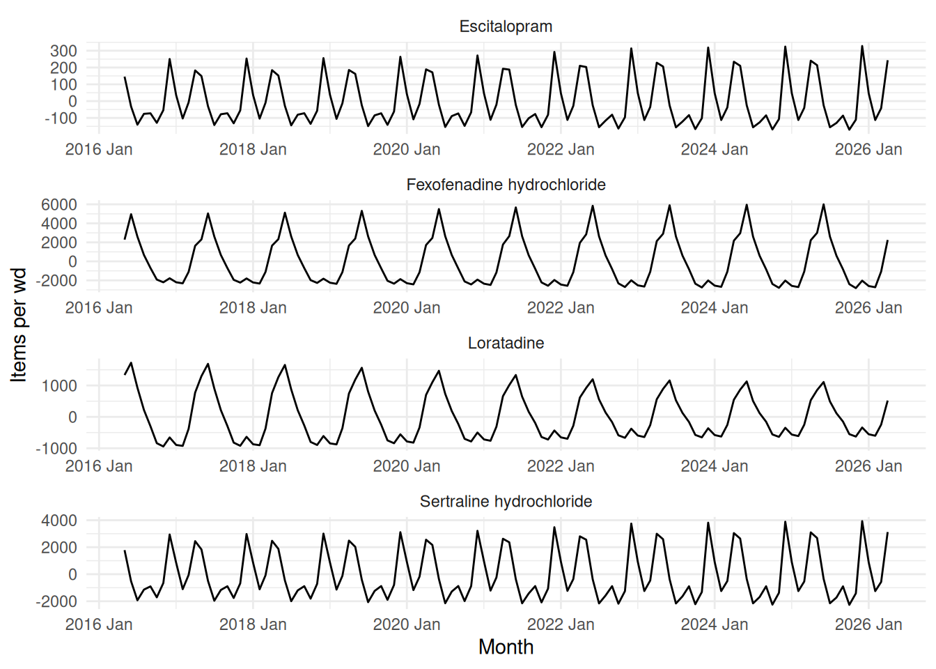
Figure 8: Plots of the pure seasonal components

FFT

Code
TOP_K <- 5
fft_scores <- score(df_detrended, top_k = TOP_K)

wrap_plots(fft_scores$plots, ncol = 2)
Figure 9: Spectral plots

Candidate periods

Code
candidates <- fft_scores$scores

write_parquet(
  candidates,
  here(TBL_DIR, glue("candidate_periods_{DETREND_TYPE}.parquet"))
)
gt(candidates)
Table 4: Candidate periods found and their signal strength from FFT (Top 5)
chemical period_1 freq_1 score_1 period_2 freq_2 score_2 period_3 freq_3 score_3 period_4 freq_4 score_4 period_5 freq_5 score_5
Loratadine 12 10 60657.688 6 20 21094.584 13.33 9 15966.179 10.91 11 14701.558 15.0 8 10346.915
Fexofenadine hydrochloride 12 10 198440.066 6 20 68348.143 3.00 40 29171.101 2.00 60 29048.628 2.4 50 23102.810
Sertraline hydrochloride 4 30 99811.825 12 10 76369.914 6.00 20 73763.278 2.31 52 32601.888 3.0 40 27239.876
Escitalopram 4 30 7883.784 6 20 6181.532 12.00 10 5617.502 2.31 52 2444.073 3.0 40 2338.871

Modelling

Code
models_results <- DF_PRESC_AGG |>
  fit_models(candidates)

write_parquet(
  models_results,
  here(TBL_DIR, glue("modelling_results_{DETREND_TYPE}.parquet"))
)

slice_head(models_results, n = 3) |> gt()
Table 5: Top 3 performing models for each chemical
.model period k lrt_stat p_value sigma2 log_lik AIC AICc BIC
0304010D0 - Loratadine
P12_K2 12 2 76.83161 <2e-16 101774.59 -852.9381 1725.876 1727.913 1753.667
K0 NA 0 NA - 201490.68 -894.2347 1800.469 1801.219 1817.144
0304010E0 - Fexofenadine hydrochloride
P12_K2 12 2 63.46607 1.7e-14 902631.08 -982.3694 1978.739 1979.748 1998.193
P12_K1 12 1 103.46077 < 2e-16 1521728.92 -1014.1024 2040.205 2040.955 2056.880
P6_K3 6 3 26.58814 1.7e-06 1750012.19 -1019.0031 2062.006 2064.950 2095.356
0403030Q0 - Sertraline hydrochloride
P12_K3 12 3 24.94745 3.8e-06 1775974.64 -1020.9344 2061.869 2063.906 2089.660
P12_K2 12 2 55.07462 1.1e-12 2172889.07 -1033.4081 2088.816 2091.283 2119.387
P4_K2 4 2 17.34475 0.00017 2884639.00 -1051.2955 2122.591 2124.628 2150.382
0403030X0 - Escitalopram
P12_K3 12 3 19.52244 5.8e-05 12797.71 -727.2842 1474.568 1476.605 1502.360
P12_K2 12 2 61.12903 5.3e-14 14928.53 -737.0455 1496.091 1498.558 1526.661
P6_K1 6 1 49.80296 1.5e-11 20878.50 -758.4120 1532.824 1534.133 1555.057

Summary report

Code
summary_tbl <- generate_report(
  ts_original = DF_PRESC_AGG,
  candidates = candidates,
  models = models_results,
  strength = strength_scores,
  top_k = TOP_K
)

write_parquet(
  summary_tbl,
  here(TBL_DIR, glue("summary_table_{DETREND_TYPE}.parquet"))
)

gt(summary_tbl) |>
  tab_header(
    title = "Seasonality Detection Summary",
    subtitle = glue(
      "Data period: {DATE_START} to {DATE_END} | Detrending: {DETREND_TYPE}"
    )
  ) |>
  fmt_number(columns = `Seasonal strength`, decimals = 2) |>
  tab_style(
    style = cell_fill(color = "#e6f2ff"),
    locations = cells_body(columns = `Model periods`)
  ) |>
  tab_footnote(
    footnote = paste0(
      "Dominant periods from FFT (strongest amplitudes), shown independently as a sanity check. ",
      "Model periods are the harmonic components (period/1, period/2, ...) actually retained ",
      "in the BIC-selected model. Peak/Trough months are the calendar months with highest/lowest ",
      "average dispensing. Best model from ARIMA errors + Fourier terms, selected by BIC. ",
      "Seasonal strength from STL decomposition."
    )
  ) |>
  tab_style(
    style = cell_text(style = "italic", size = px(12)),
    locations = cells_footnotes()
  )
Seasonality Detection Summary
Data period: 2016-05-01 to 2026-04-01 | Detrending: stl
Chemical Dominant periods (FFT) Model periods Peak month Trough month Seasonal strength Best model LRT p-value
Escitalopram 4, 6, 12 12, 6, 4 Dec Oct 0.80 P12_K3 (P=12, K=3) 5.8e-05
Fexofenadine hydrochloride 12, 6, 3 12, 6 Jun Nov 0.96 P12_K2 (P=12, K=2) 1.7e-14
Loratadine 12, 6, 13.3 12, 6 Jun Nov 0.91 P12_K2 (P=12, K=2) <2e-16
Sertraline hydrochloride 4, 12, 6 12, 6, 4 Dec Oct 0.79 P12_K3 (P=12, K=3) 3.8e-06
Dominant periods from FFT (strongest amplitudes), shown independently as a sanity check. Model periods are the harmonic components (period/1, period/2, ...) actually retained in the BIC-selected model. Peak/Trough months are the calendar months with highest/lowest average dispensing. Best model from ARIMA errors + Fourier terms, selected by BIC. Seasonal strength from STL decomposition.

References

1. Richardson, N., Cook, I., Crane, N., Dunnington, D., François, R., Keane, J., Mecum, B., Moldovan-Grünfeld, D., Ooms, J., Wujciak-Jens, J., & Apache Arrow. (2026). Arrow: Integration to apache ’arrow’. https://github.com/apache/arrow/
2. Freitas, W. (2025). Bizdays: Business days calculations and utilities. https://github.com/wilsonfreitas/R-bizdays
3. Hyndman, R. (2026). fpp3: Data for "forecasting: Principles and practice" (3rd edition). https://pkg.robjhyndman.com/fpp3/
4. Slowikowski, K. (2026). Ggrepel: Automatically position non-overlapping text labels with ggplot2. https://ggrepel.slowkow.com/
5. Hester, J., & Bryan, J. (2026). Glue: Interpreted string literals. https://glue.tidyverse.org/
6. Iannone, R., Cheng, J., Schloerke, B., Haughton, S., Hughes, E., Lauer, A., Fran?ois, R., Seo, J., Brevoort, K., & Roy, O. (2026). Gt: Easily create presentation-ready display tables. https://gt.rstudio.com
7. Müller, K. (2025). Here: A simpler way to find your files. https://here.r-lib.org/
8. Pedersen, T. L. (2025). Patchwork: The composer of plots. https://patchwork.data-imaginist.com
9. Wickham, H., & Henry, L. (2026). Purrr: Functional programming tools. https://purrr.tidyverse.org/
10. Wickham, H. (2023). Tidyverse: Easily install and load the tidyverse. https://tidyverse.tidyverse.org
11. Wuertz, D., Setz, T., Chalabi, Y., & Boshnakov, G. N. (2026). timeDate: Rmetrics - chronological and calendar objects. https://geobosh.github.io/timeDateDoc/
12. Pfaff, B. (2024). Urca: Unit root and cointegration tests for time series data.
13. Chang, W. (2025). webshot2: Take screenshots of web pages. https://rstudio.github.io/webshot2/
14. Wickham, H., Averick, M., Bryan, J., Chang, W., McGowan, L. D., François, R., Grolemund, G., Hayes, A., Henry, L., Hester, J., Kuhn, M., Pedersen, T. L., Miller, E., Bache, S. M., Müller, K., Ooms, J., Robinson, D., Seidel, D. P., Spinu, V., … Yutani, H. (2019). Welcome to the tidyverse. Journal of Open Source Software, 4(43), 1686. https://doi.org/10.21105/joss.01686
15. Pfaff, B. (2008). Analysis of integrated and cointegrated time series with r (Second). Springer. https://www.pfaffikus.de