Understanding Seasonal Patterns in NHS Prescribing Data

1 Introduction

This project investigates seasonal patterns in prescribing in English primary care using routinely collected NHS prescribing data from OpenPrescribing. The analysis examines a selection of medicines with expected seasonal and non-seasonal prescribing patterns, using visual and statistical time-series methods to identify recurring changes over time.

The analysis combines seasonal visualisations (gg_season() and gg_subseries()) with STL decomposition to separate longer-term trends from recurring seasonal variation. The aim is to explore how clearly seasonal patterns can be identified in prescribing data and how these patterns should be interpreted in the context of real-world clinical and temporal factors.

2 Research question

Can recurring seasonal patterns in prescribing be identified and meaningfully interpreted from routinely collected NHS prescribing data?

3 Setup

Load packages and set up variables for BNF codes and data date range (January 2015 to December 2025)

# library(opr)
library(tidyverse)
library(scales)
library(gt)
library(here)
library(arrow)
library(tsibble)
library(feasts)
library(ggrepel)
library(patchwork)

Connect to BigQuery. See here.

con <- connect_bq()

4 Data extraction

Prescribing data were obtained from OpenPrescribing, which provides routinely collected NHS prescribing data for England.

Data were extracted at the BNF chemical level for the medicines included in the analysis. Monthly prescribing volumes were used to examine changes over time.

bnf_code_amoxicillin <- "0501013B0%"
bnf_code_phenoxymethylpenicillin <- "0501011P0%"
bnf_code_clarithromycin <- "0501050B0%"
bnf_code_cetirizine <- "0304010I0%"
bnf_code_fexofenadine <- "0304010E0%"

## negative controls — drugs with expected minimal/no seasonality
bnf_code_mesalazine <- "0105010B0%"
bnf_code_tamoxifen <- "0803041S0%"
bnf_code_finasteride <- "0604020C0%"

df_prescribing <- get_normalised_prescribing(
  con,
  bnf_codes = c(bnf_code_amoxicillin,
  bnf_code_phenoxymethylpenicillin,
  bnf_code_clarithromycin,
  bnf_code_cetirizine,
  bnf_code_fexofenadine,
  bnf_code_mesalazine,
  bnf_code_tamoxifen,
  bnf_code_finasteride),
  start_date = "2015-01-01",
  end_date = "2025-12-31"
) |>
  select(
    month,
    practice,
    regional_team,
    items,
    stp,
    bnf_code,
    bnf_name
  ) 

  db_chemicals <- tbl(con, "bnf") |>
  select(presentation_code, chemical)

df_prescribing <- df_prescribing  |>
  inner_join(db_chemicals, by = c("bnf_code" = "presentation_code"))   |>
collect()

df_practices <- get_practices(con, filter_setting = 4) |>
  collect()

df_regional_teams <- tbl(con, "regional_teams") |>
  collect()

## add list size to table from "practice_statistics"
df_list_size <- tbl(con, "practice_statistics") |>
  select(practice, month, total_list_size) |>
  collect()


write_parquet(
  df_prescribing,
  here("data-raw", "najma", "df_prescribing.parquet")
)

write_parquet(
  df_practices,
  here("data-raw", "najma", "df_practices.parquet")
)

write_parquet(
  df_regional_teams,
  here("data-raw", "najma", "df_regional_teams.parquet")
)

write_parquet(
  df_list_size,
  here("data-raw", "najma", "df_list_size.parquet")
)

The extraction produced a monthly time series for each medicine, providing the basis for subsequent seasonal analysis.

df_prescribing <- read_parquet(
  here("data-raw", "najma", "df_prescribing.parquet")
)

df_practices <- read_parquet(
  here("data-raw", "najma", "df_practices.parquet")
)

df_regional_teams <- read_parquet(
  here("data-raw", "najma", "df_regional_teams.parquet")
)

df_list_size <- read_parquet(
  here("data-raw", "najma", "df_list_size.parquet")
)

5 Data Normalisation

Prescribing counts are normalised by practice list size, shown as items per 1000 registered patients per month. This is to account for raw prescribing item counts not being directly comparable across practices over time due to differences in list sizes.

Practice-level list size data is drawn from practice_statistics and joined to the prescribing data by practice and month.

df_prescribing_normalised <- df_prescribing |>
  left_join(df_list_size, by = c("practice", "month"))

## compute practice-level rate
## kept at practice level (not yet aggregated) so it can be joined
## to a region lookup later for the regional variation extension
df_prescribing_normalised <- df_prescribing_normalised |>
  mutate(rate_per_1000 = items / total_list_size * 1000)

## aggregate data (national level, for the primary seasonality analysis)

df_monthly_items <- df_prescribing |>
  group_by(chemical, month) |>
  summarise(items = sum(items), .groups = "drop")

df_monthly_list_size <- df_list_size |>
  group_by(month) |>
  summarise(total_list_size = sum(total_list_size), .groups = "drop")

df_monthly_rate <- df_monthly_items |>
  left_join(df_monthly_list_size, by = "month") |>
  mutate(rate_per_1000 = items / total_list_size * 1000)

## convert date for tsibble

df_monthly_rate <- df_monthly_rate |>
  mutate(month = yearmonth(as.Date(month)))

6 Visual Seasonality Assessment

6.1 Seasonal Plots

Before applying any quantitative measure, we first inspect seasonality visually using gg_season(), which plots each year’s data as a separate line across the months of the year. This lets us see, by eye, whether a drug’s prescribing consistently peaks or troughs in the same months year after year ,as opposed to a one-off spike or a gradual trend.

df_monthly_rate_tsibble <- df_monthly_rate |>
  mutate(month = yearmonth(month)) |>
  as_tsibble(index = month, key = chemical)

drugs <- unique(df_monthly_rate_tsibble$chemical)

## split into expected-seasonal (benchmark) vs expected-flat (negative control) groups
negative_controls <- c("Mesalazine (Systemic)", "Tamoxifen citrate", "Finasteride")
benchmark_drugs <- setdiff(drugs, negative_controls)

## building list of plots instead of printing each one individually
plot_list1 <- purrr::map(drugs, function(d) {
  
  df_monthly_rate_tsibble |>
    filter(chemical == d) |>
    gg_season(rate_per_1000, labels = "right", labels_repel = TRUE) +
    labs(
      title = d,
      y = "Items per 1,000 registered patients",
      x = NULL
    )
})
names(plot_list1) <- drugs

## combine benchmark (expected seasonal) drugs into one figure
combined_plot1_benchmark <- wrap_plots(plot_list1[benchmark_drugs], ncol = 2) +
  plot_annotation(title = "Expected seasonal (benchmark drugs)")

## combine negative control (expected flat) drugs into one figure
combined_plot1_negative <- wrap_plots(plot_list1[negative_controls], ncol = 2) +
  plot_annotation(title = "Expected minimal/no seasonality (negative controls)")

combined_plot1_benchmark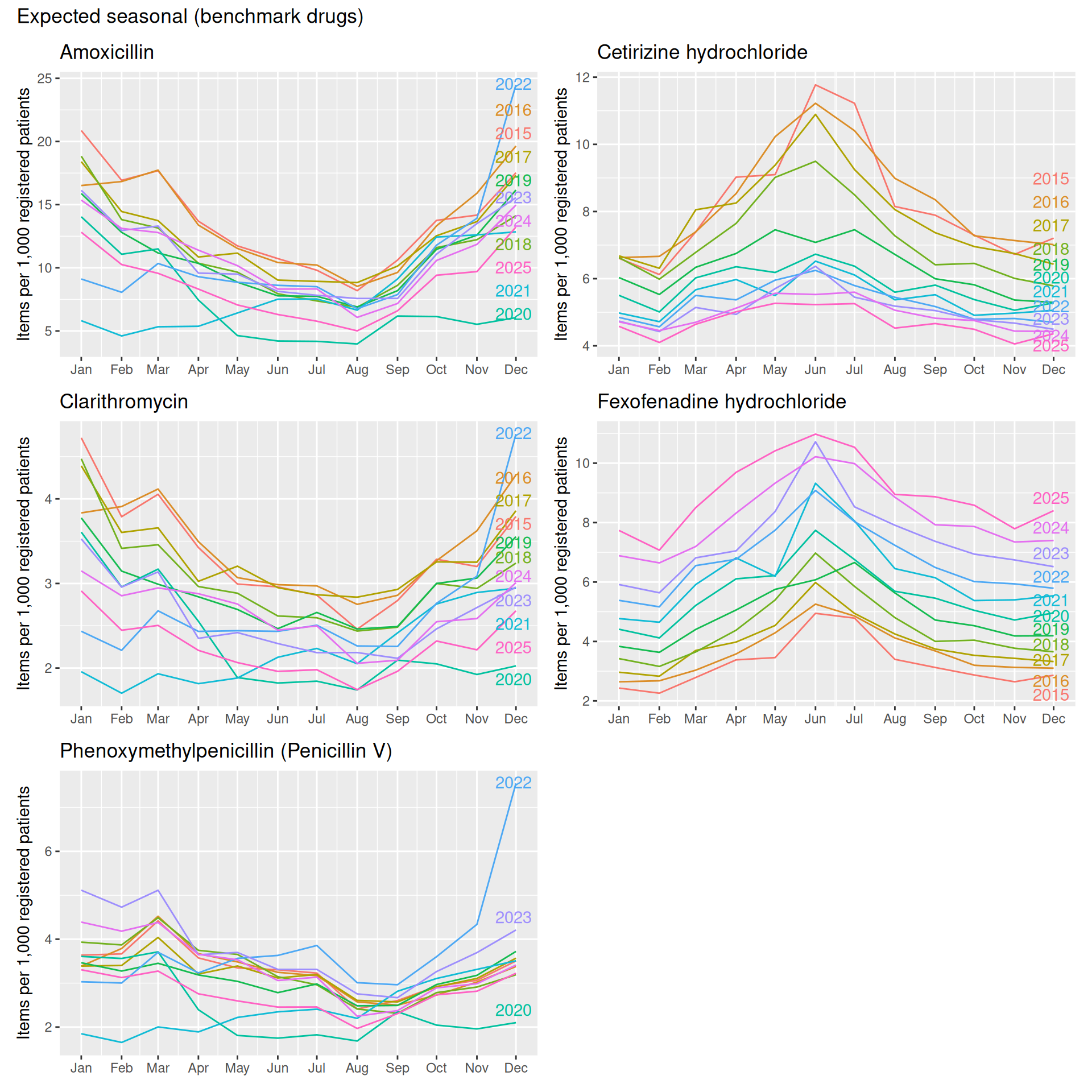

Figure 1

combined_plot1_negative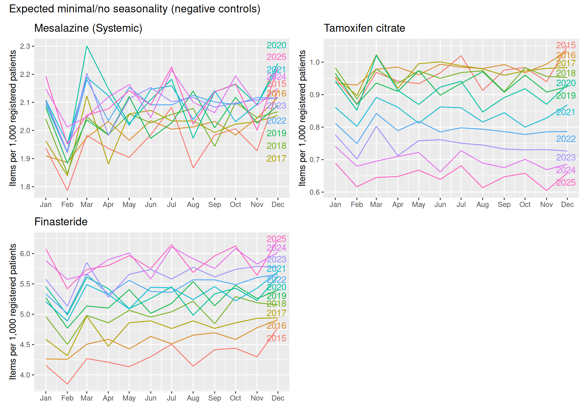

Figure 2

6.1.1 Findings:

gg_season() plots display distinct visual seasonality for most of the positive controls. Amoxicillin shows a strong and consistent winter peak (Dec-Jan) and summer trough (Jul-Aug) across nearly every year bar 2020, a distinct anomaly. Clarithromycin follows a similar pattern, though with more year-to-year noise, especially in 2020-2021. Cetrizine and Fexofenadine show the cleanest seasonal signals of all the drugs, with consistent, low-noise summer peaks in June.

Phenxomethylpenicllin is the weakest positive control visually, with a much smaller seasonal amplitude than the other antibiotics and a much less consistent shape (a modest March peak rather than a clean winter peak) and a large anomalous spike in December 2022, which can be attributed to the UK Strep A outbreak. The March peaks reflect calendar effects (i.e. working-day counts) rather than a genuine seasonal driver. This weakens the case for Phenoxymethylpenicillin as a strong seasonal benchmark.

The negative controls displayed no consistent recurring shape. Mesalazine had considerable monthly variation with no stable pattern across the years. Tamoxifen and Finasteride were both dominated by long-term strong trends, rather than any meaningful seasonal cycle.

6.2 Subseries Plots

As a complementary view, gg_subseries() groups all observations by month (all Januaries together, all Februaries together, etc.) and shows the average level for each month as a horizontal reference line. This makes it easier to spot whether certain months are systematically higher or lower across the whole time series, independent of year-to-year trend or noise that can make the gg_season() plot harder to read.

## building list of subseries plots
plot_list2 <- purrr::map(drugs, function(d) {
  
  df_monthly_rate_tsibble |>
    filter(chemical == d) |>
    gg_subseries(rate_per_1000) +
    labs(
      title = d,
      y = "Items per 1,000 registered patients",
      x = NULL
    )
})
names(plot_list2) <- drugs

## combine benchmark (expected seasonal) drugs into one figure
combined_plot2_benchmark <- wrap_plots(plot_list2[benchmark_drugs], ncol = 1) +
  plot_annotation(title = "Expected seasonal (benchmark drugs)")

combined_plot2_benchmark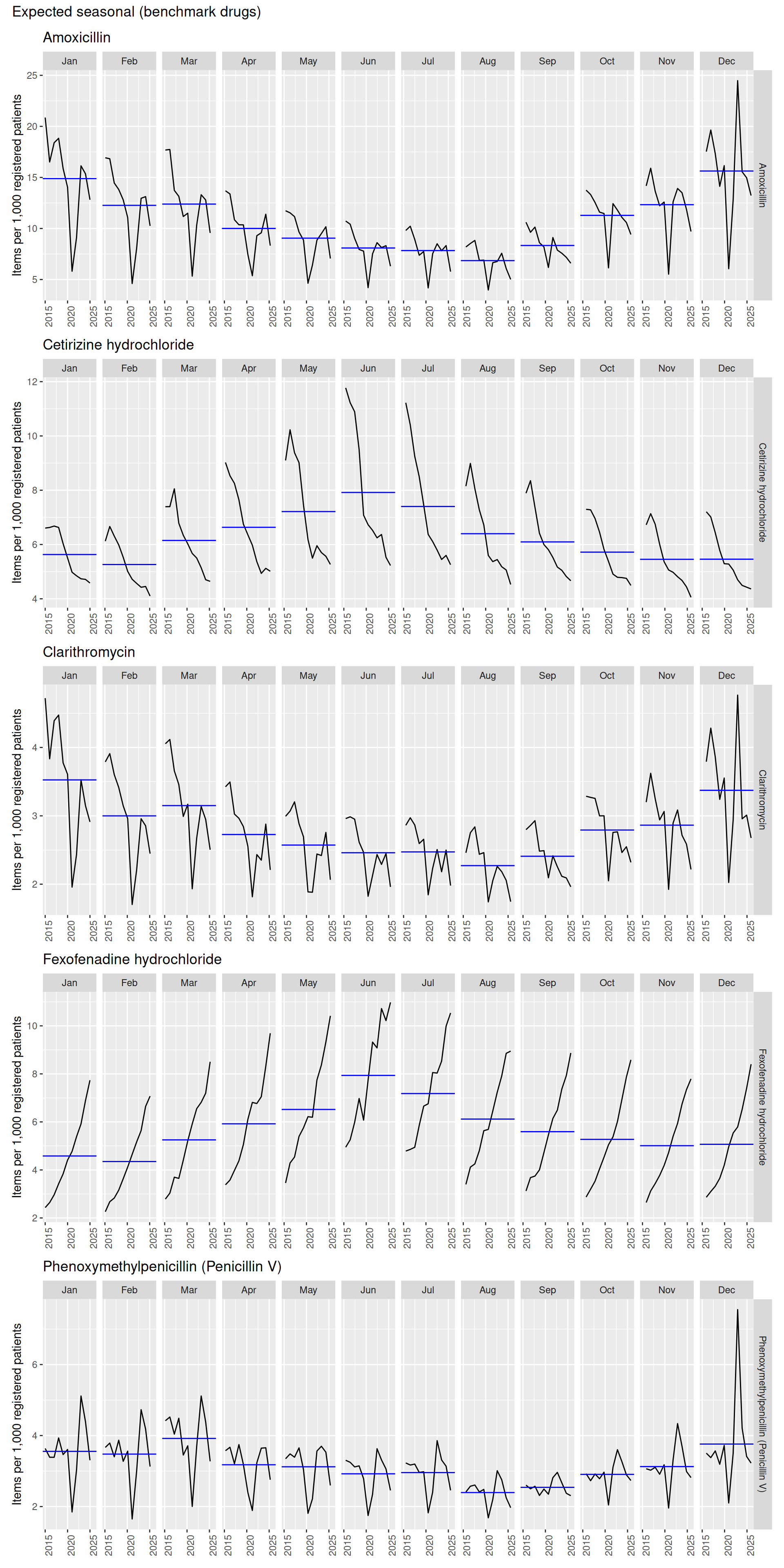

Figure 3

## combine negative control (expected flat) drugs into one figure
combined_plot2_negative <- wrap_plots(plot_list2[negative_controls], ncol = 1) +
  plot_annotation(title = "Expected minimal/no seasonality (negative controls)")

combined_plot2_negative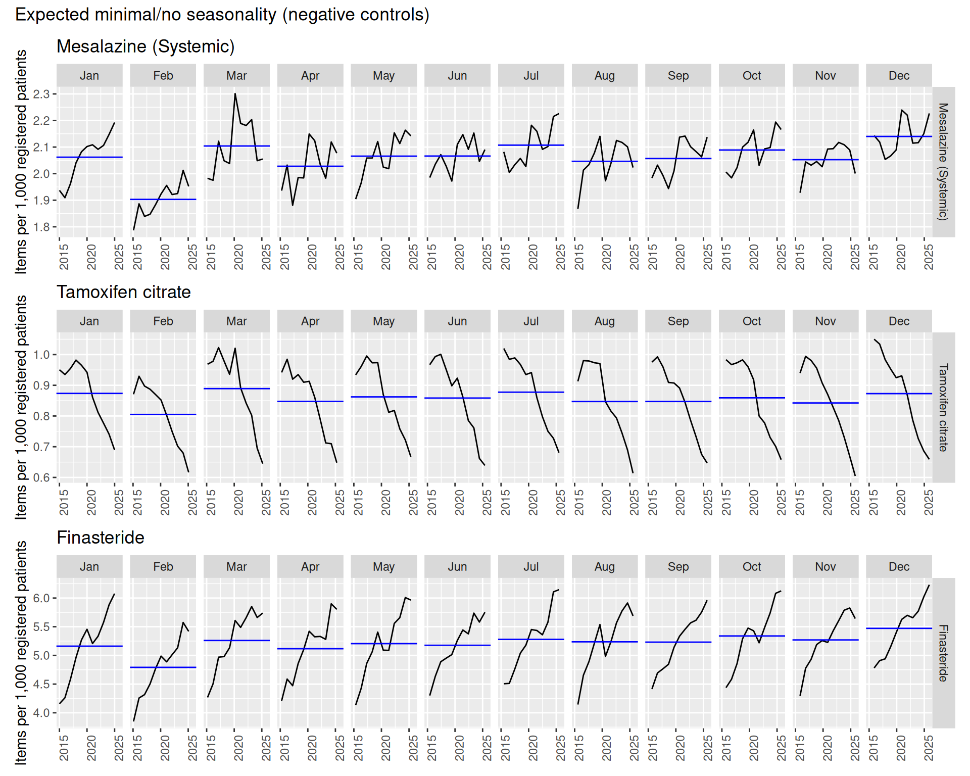

Figure 4

6.2.1 Findings

The subseries plots displayed similar findings to the gg_season() graphs, with a few distinct additional findings. Cetirizine showed a pronounced downward trend across individual months, indicating that its apparent seasonal pattern occurred alongside a long-term decline in prescribing. In contrast, fexofenadine showed a recurring seasonal pattern alongside an increase in prescribing over time. This highlights how recurring seasonal patterns can coexist with substantial longer-term changes in prescribing.

6.3 Save Visual Assessment Figures

Individual gg_season() and gg_subseries() plots for each control drug are combined into four composite figures using the patchwork package, and saved for reference.

ggsave(
    filename = here("outputs", "figures", "najma", "gg_season_all_benchmarks.png"),
    plot = combined_plot1_benchmark,
    height = 10,
    width = 10
  )

ggsave(
    filename = here("outputs", "figures", "najma", "gg_season_all_negative.png"),
    plot = combined_plot1_negative,
    height = 7,
    width = 10
  )

ggsave(
    filename = here("outputs", "figures", "najma", "gg_subseries_all_benchmarks.png"),
    plot = combined_plot2_benchmark,
    height = 20,
    width = 10
  )

  ggsave(
    filename = here("outputs", "figures", "najma", "gg_subseries_all_negative.png"),
    plot = combined_plot2_negative,
    height = 8,
    width = 9
  )

7 STL-Based Seasonal Strength Scoring

Having visually assessed seasonality, we now turn to a quantitative measure: seasonal strength scores derived from STL (Seasonal-Trend decomposition using Loess), calculated via feat_stl() from the feasts package. This decomposes each time series into trend, seasonal, and remainder components, and computes a seasonal strength score (Wang et al, 2006) reflecting how much of the variation in the series is explained by the seasonal component relative to noise.

The aim here is to test whether this single quantitative score can reliably distinguish the known-seasonal benchmark drugs from the non-seasonal ones, and whether it adds meaningful information beyond what visual inspection alone already showed.

formatted_decimal <- function(number) {
  format(number, big.mark = ",", scientific = FALSE, digits = 3)
}

## compute seasonal/trend strength scores for all drugs at once
df_feat_stl <- df_monthly_rate_tsibble |>
  features(rate_per_1000, feat_stl)

df_feat_stl |>
  mutate(across(where(is.numeric), formatted_decimal)) |>
  gt() |>
  cols_align(
    align = "center",
    columns = everything()
  )

Seasonal score for select drugs

chemical	trend_strength	seasonal_strength_year	seasonal_peak_year	seasonal_trough_year	spikiness	linearity	curvature	stl_e_acf1	stl_e_acf10
Amoxicillin	0.756	0.811	0	8	0.0016699465021	-15.252	10.888	0.504	0.576
Cetirizine hydrochloride	0.935	0.868	6	2	0.0000051553981	-14.588	2.470	0.317	0.603
Clarithromycin	0.818	0.750	1	8	0.0000012993218	-4.107	1.359	0.430	0.416
Fexofenadine hydrochloride	0.981	0.942	6	2	0.0000012620480	20.836	2.400	-0.173	0.201
Finasteride	0.939	0.510	0	2	0.0000000187188	5.536	-0.776	-0.509	0.999
Mesalazine (Systemic)	0.525	0.550	0	2	0.0000000006028	0.542	-0.196	-0.456	0.644
Phenoxymethylpenicillin (Penicillin V)	0.711	0.624	0	8	0.0000173899107	-0.184	0.949	0.456	0.481
Tamoxifen citrate	0.968	0.553	0	2	0.0000000000246	-1.246	-0.378	-0.466	0.574

7.1 Findings:

Taking the threshold of 0.64 (Hyndman RJ, Athanasopoulos G., 2021) into account, the positive controls behaved as expected: Amoxicillin (0.811), clarithromycin (0.750), cetirizine (0.868) and fexofenadine (0.942) all scored above the threshold. This aligns with the winter and summer seasonal patterns observed in the prior visual assessment. However, phenoxymethylpenicillin (0.64) fell below the threshold despite it being a known seasonal drug.

This highlights a limitation of applying this threshold. The 0.64 cutoff origniates from nsdiffs(), an ARIMA differencing heuristic, rather than a threshold used for distinguishing seasonal from non-seasonal drugs. Its use should there be treated cautiously rather than a definitive classificati

As expected, all three negative controls scored below the threshold: mesalazine (0.550), tamoxifen (0.553) and finasteride (0.510).

7.2 Visualising the STL decomposition

We plot the full decomposition for both the positive and negative controls to understand what the strength score is actually capturing. This displays the original series alongside its trend, seasonal and remainder components (separated). This could help identify possible outliers, trend shifts etc. that could influence the seasonal strength score.

## STL for every drug at once
df_stl_components <- df_monthly_rate_tsibble |>
  model(STL(rate_per_1000 ~ season(window = "periodic"))) |>
  components()

## helper function to build decomposition plots for a given set of drugs
build_stl_plots <- function(drug_names) {
  purrr::map(drug_names, function(d) {
    df_stl_components |>
      filter(chemical == d) |>
      autoplot() +
      labs(title = d) +
      theme_minimal(base_size = 8) +
      theme(strip.text = element_text(size = 7))
  }) |>
    purrr::compact()
}

plot_list3_benchmark <- build_stl_plots(benchmark_drugs)
plot_list3_negative <- build_stl_plots(negative_controls)

combined_plot3_benchmark <- wrap_plots(plot_list3_benchmark, ncol = 1) +
  plot_annotation(title = "STL decomposition — expected seasonal (benchmark drugs)")

combined_plot3_negative <- wrap_plots(plot_list3_negative, ncol = 1) +
  plot_annotation(title = "STL decomposition — expected minimal/no seasonality (negative controls)")

combined_plot3_benchmark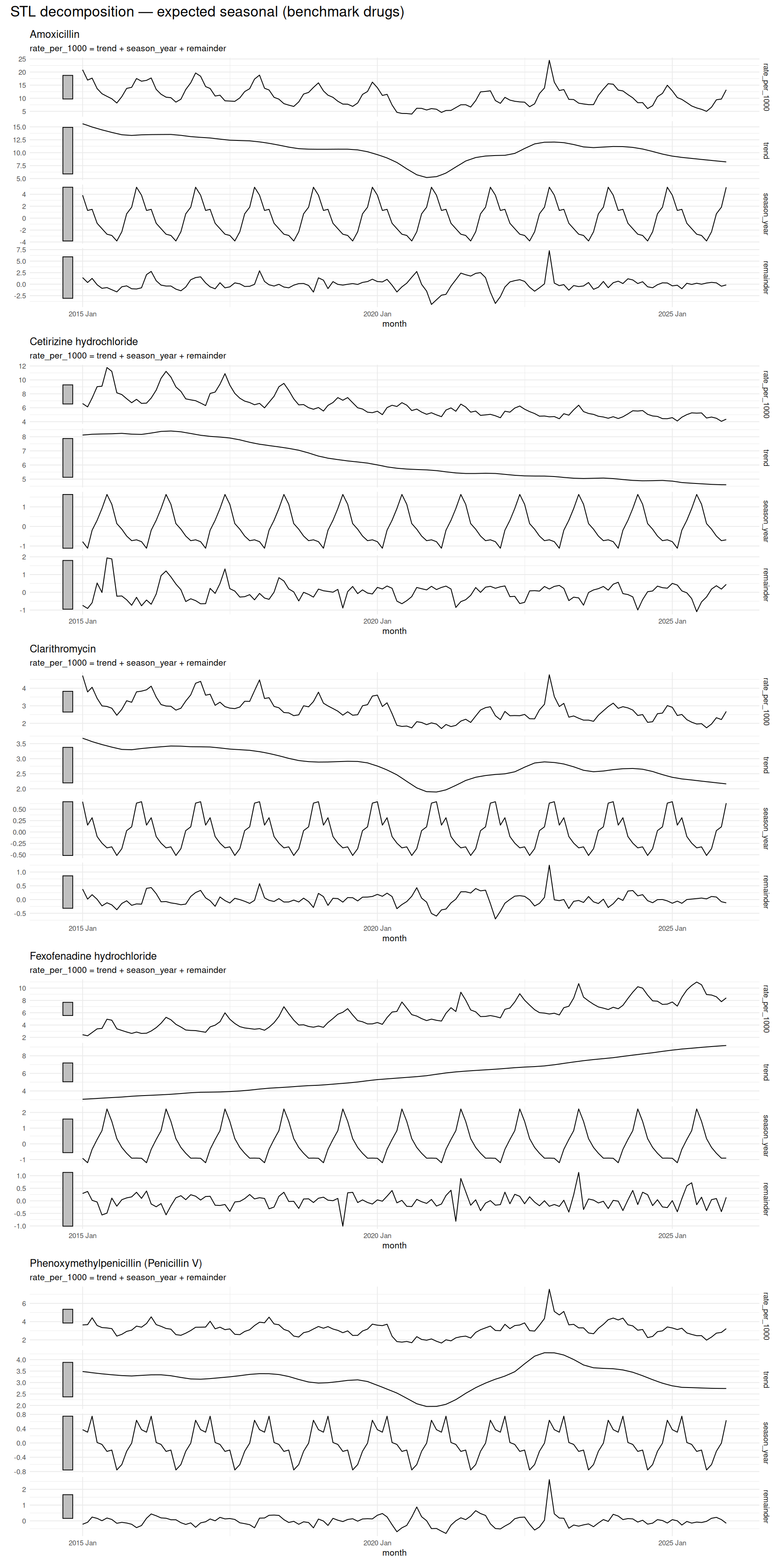

Figure 5

STL allowed the recurring seasonal component to be separated from longer-term trends and unusual fluctuations. This highlighted that a statistical seasonal component does not necessarily correspond straightforwardly to clinically meaningful seasonality, particularly for the negative controls.

combined_plot3_negative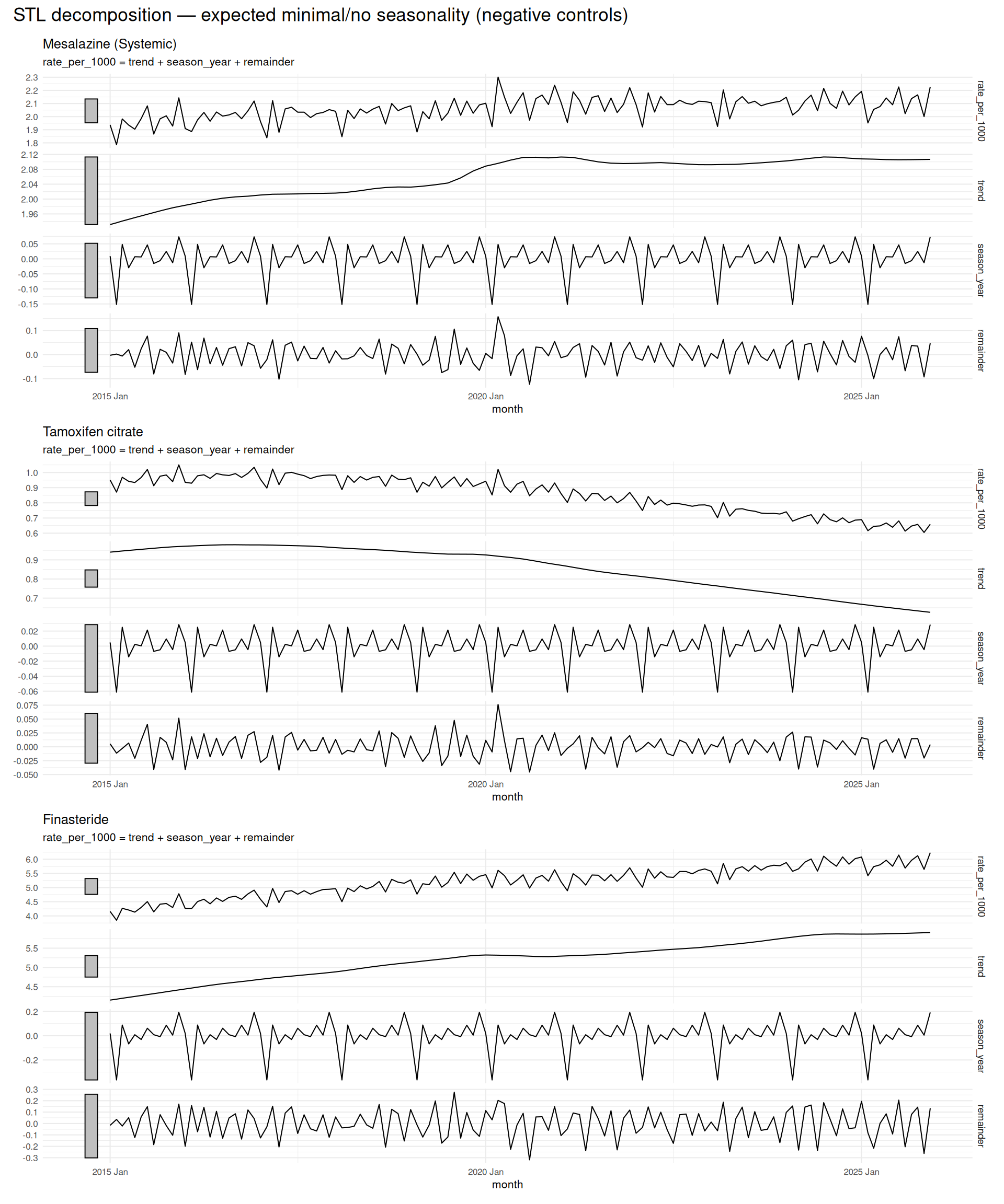

Figure 6

7.2.1 Save STL Decomposition figures

Like the gg_season() figures, these STL decompositions plots are combined into two plots (separated by positive and negative), allowing for comparison against the prior visual assessment.

ggsave(
    filename = here("outputs", "figures", "najma", "feats_stl_all_benchmarks.png"),
    plot = combined_plot3_benchmark,
    height = 20,
    width = 10
  )

  ggsave(
    filename = here("outputs", "figures", "najma", "feasts_stl_all_negative.png"),
    plot = combined_plot3_negative,
    height = 12,
    width = 10
  )