Extract semantic tags from SNOMED CT descriptions

SNOMED CT descriptions include semantic tags in parentheses that classify concepts into categories such as (procedure), (finding), (observable entity), or (disorder). Understanding these tags helps researchers interpret what types of clinical activities their codelists capture. For example, a depression screening codelist might include procedures (the act of screening), observable entities (measurable scores), and findings (clinical conclusions).

Worked example

In this example we’re looking at the Depression screening codes (DEPSCRN_COD) from the NHS Primary Care Domain Reference Set Portal:

Setup

# Load packages
library(opencodecounts)
library(dplyr)
library(stringr)
library(ggplot2)
library(scales)
library(gt)

# Load code extract semantic tag
depscrn_cod <- get_codelist(
  "nhsd-primary-care-domain-refsets/depscrn_cod/20250627"
)

# Get data for both codelists and extract semantic tag
depscrn_cod_usage <- snomed_usage |>
  filter(snomed_code %in% c(depscrn_cod$code)) |>
  mutate(
    semantic_tag = extract_semantic_tag(description),
    semantic_tag = str_to_sentence(semantic_tag),
    description_short = strip_semantic_tag(description),
  )

Table with most used codes

# Calculate sum by code for entire time period
df_tab_top10_depscrn_cod <- depscrn_cod_usage |>
  group_by(snomed_code, description_short, semantic_tag) |>
  summarise(total_usage = sum(usage), .groups = 'drop') |>
  mutate(ratio_usage = total_usage / sum(total_usage)) |> 
  slice_max(order_by = total_usage, n = 10)

# Create table
df_tab_top10_depscrn_cod |>
  group_by(semantic_tag) |>
  gt() |>
  cols_label(
    snomed_code = "SNOMED code",
    description_short = "Description",
    total_usage = "Usage",
    ratio_usage = "%"
  ) |>
  tab_style(
    style = cell_text(weight = "bold"),
    locations = cells_column_labels()
  ) |>
  tab_style(
    style = cell_text(font = "Courier New"),
    locations = cells_body(columns = snomed_code)
  ) |>
  cols_align(align = "left", columns = snomed_code) |>
  fmt_number(total_usage, decimals = 0) |>
  fmt_percent(ratio_usage, decimals = 2)

SNOMED code	Description	Usage	%
Procedure
200971000000100	Depression screening using questions	21,510,040	54.46%
171207006	Depression screening	609,620	1.54%
792491000000100	Assessment using Whooley depression screen	122,830	0.31%
715252007	Depression screening using Patient Health Questionnaire Nine Item score	25,760	0.07%
Observable entity
720433000	Patient Health Questionnaire Nine Item score	16,229,920	41.09%
401320004	Hospital Anxiety and Depression scale: depression score	790,280	2.00%
450320001	Edinburgh postnatal depression scale score	146,120	0.37%
718366000	Beck Depression Inventory II score	43,340	0.11%
803351000000106	Whooley depression screen score	7,010	0.02%
Finding
112011000119102	Negative screening for depression on Patient Health Questionnaire 9	7,620	0.02%

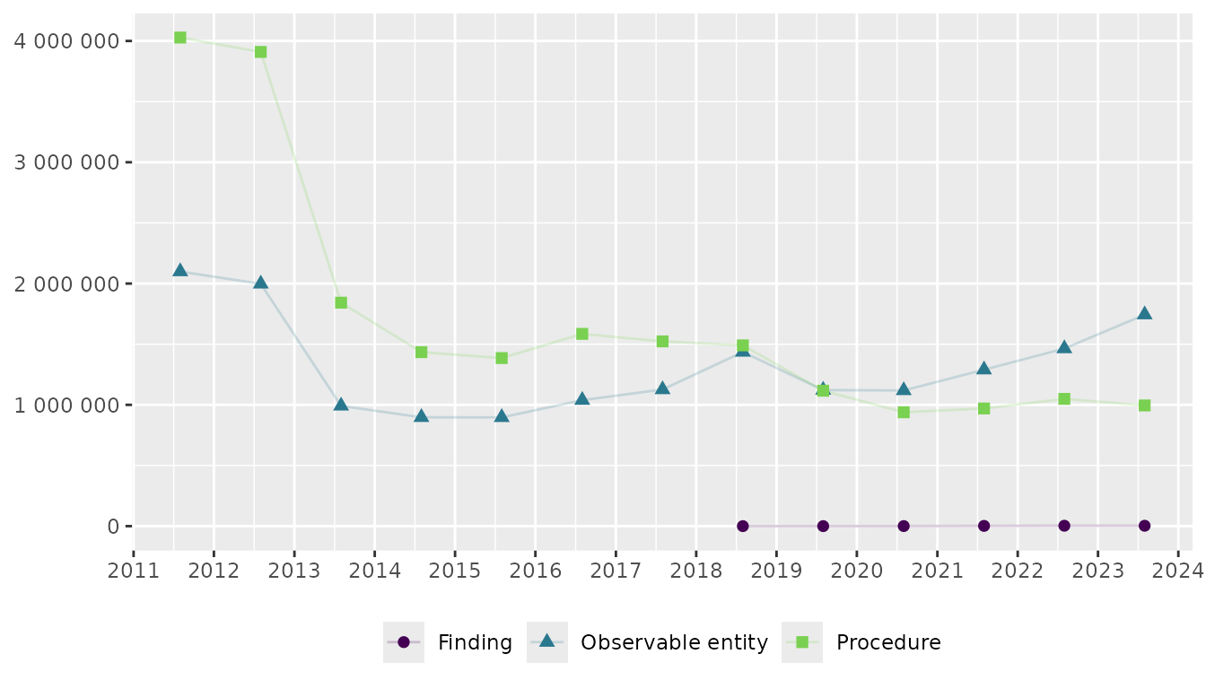
Figure showing trends over time by semantic tag

# Calculate yearly sum by semantic tag
df_fig_sem_tag_depscrn_cod <- depscrn_cod_usage |>
  group_by(start_date, semantic_tag) |>
  summarise(total_usage = sum(usage), .groups = 'drop')

# Create figure
df_fig_sem_tag_depscrn_cod |>
  ggplot(
    aes(
      y = total_usage,
      x = start_date,
      colour = semantic_tag,
      shape = semantic_tag
    )
  ) +
  geom_line(alpha = 0.2) +
  geom_point(size = 2) +
  labs(title = NULL, x = NULL, y = NULL, colour = NULL, shape = NULL) +
  scale_x_date(date_breaks = "1 year", labels = label_date_short()) +
  scale_y_continuous(labels = label_number(accuracy = 1), limits = c(0, NA)) +
  theme(legend.position = "bottom") +
  scale_colour_viridis_d(end = .8)